Basics of Using a Stored Procedure With Db2 Web Query for i Version 2.3

The most recent releases of Db2 Web Query introduced interface enhancements to the Home page, metadata management and report design. This article will discuss some of these changes in the context of illustrating using an SQL stored procedure (SP) as a data source for one or more Web Query reports. The procedure presents data for which WQ metadata can define a drill-down hierarchy. This will highlight the power of the SP, showcasing the Home page, the Metadata editor and reports using data from the SP.

Overview of the SP

SPs are SQL programs which offer a way to provide information to consuming applications. Db2 Web Query can act as a consumer of such data. You create the procedure, then tell WQ it exists, much as you would with any Db2 table or view.

Let’s examine some procedure definition code and the creation process. The steps to create the procedure are:

• Open ACS
• Start Run SQL Scripts
• Write (or paste) the code to define your SP (in my case named DASH5)
• Run the CREATE PROCEDURE statement
• Test the procedure by “calling” DASH5

On the Create Procedure statement I named the procedure DASH5( ). This procedure doesn’t require input parameters, but if it had, they’d be coded between the parens following the name. Because this procedure returns TWO results, we must code Dynamic Result Sets 2. And of course, because this is SQL, we say Language SQL. We follow that with the Declare statements.

Tip: Test SELECT statement(s) individually before placing the code in the Procedure definition.

This procedure declares two cursors, C1 and C2 to return two result sets for WQ. In the code segment, each DECLARE uses a common table expression to extract some basic data from tables in QWQCENT Library and then summarizes that data.

C1 declares selection of geographic fields, time periods and summarizes dollars for revenue, cost and profit.

C2 declares selection of product fields, time periods and summarizes the same three dollar fields.

As you can see, these geography and product fields used for grouping are organized from high-to-low in terms of detail. These will become the WQ hierarchies in the metadata. Also, date information is included which could be useful for charting trend over time information.

Following the Declares, we must OPEN each cursor. Finally we set each result set to a cursor. This essentially provides pointers to the returned data so that WQ or another process can consume it.

When the procedure has been created, we can use the SQL CALL command in ACS Run SQL Scripts, to test the Procedure to verify it produces the desired result set windows.

Example call: CALL DASH5( );

— Begin procedure code


-- SP to compare this year, by month to last year, with yr-over-yr $ 


CREATE OR REPLACE PROCEDURE Dash5()

    DYNAMIC RESULT SETS 2

    LANGUAGE SQL

    BEGIN


 DECLARE C1 CURSOR FOR

 WITH a

  AS (SELECT country,region, state, city, YEAR(orderdate) AS ordYY, MONTH(orderdate) AS ordM, MONTHNAME(orderdate)

         AS ordMn,          (LINETOTAL * QUANTITY) AS REVENUE,

         (costofgoodssold * QUANTITY) AS Extcost,

         (LINETOTAL * QUANTITY) - (costofgoodssold * QUANTITY) AS ExtProfit

        FROM qwqcent.orders o join qwqcent.stores s on o.storecode = s.storecode )

  SELECT country,region, state, city, ordYY, ordYY || '-' || SUBSTR(DIGITS(ordM), 9, 2) as Period, ordMn , 

  sum(revenue) AS PeriodRev,

    sum(ExtCost) AS PeriodCost ,

      sum(ExtProfit) AS PeriodProfit  

  FROM a 

  GROUP BY country,region, state, city, ordYY, ordYY || '-' || SUBSTR(DIGITS(ordM), 9, 2) , ordMn 

  ORDER BY country,region, state, city, ordYY, ordYY || '-' || SUBSTR(DIGITS(ordM), 9, 2) , ordMn DESC ; 



DECLARE C2 CURSOR FOR   

WITH a

  AS (SELECT ProductType, ProductCategory, ProductName, Model, o.productNumber, YEAR(orderdate) AS ordYY, MONTH(orderdate) AS ordM, MONTHNAME(orderdate)

         AS ordMn,          (LINETOTAL * QUANTITY) AS REVENUE,

         (costofgoodssold * QUANTITY) AS Extcost,

         (LINETOTAL * QUANTITY) - (costofgoodssold * QUANTITY) AS ExtProfit

        FROM qwqcent.orders o join qwqcent.inventory i on o.productnumber = i.productnumber )

  SELECT ProductType, ProductCategory, ProductName, Model, productNumber, 

  ordYY || '-' || SUBSTR(DIGITS(ordM), 9, 2) as Period, ordMn , 

  sum(revenue) AS PeriodRev,

    sum(ExtCost) AS PeriodCost ,

      sum(ExtProfit) AS PeriodProfit  

  FROM a 

  GROUP BY ProductType, ProductCategory, ProductName, Model, productNumber, ordYY || '-' || SUBSTR(DIGITS(ordM), 9, 2) , ordMn 

  ORDER BY ProductType, ProductCategory, ProductName, Model, productNumber, ordYY || '-' || SUBSTR(DIGITS(ordM), 9, 2) , ordMn DESC;


  OPEN C1;

  OPEN C2;

  SET RESULT SETS CURSOR C1,CURSOR C2;

END;        

       

— End procedure code

Overview of the Old and New WQ Interfaces

Figure 1 shows the Db2 Web Query for i home page in Version 2.2.1, where reports you have authored or have access to, are listed by name. Reports are often grouped by subject in folders. This is the main Home page where report consumers are able to run reports.

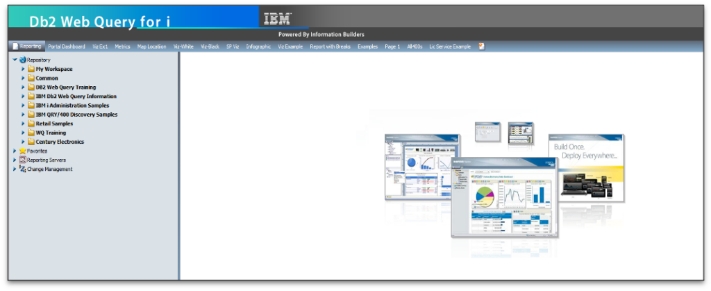
Figure 2 shows the release V2.3 home page interface, initially displaying recent work or your favorites.

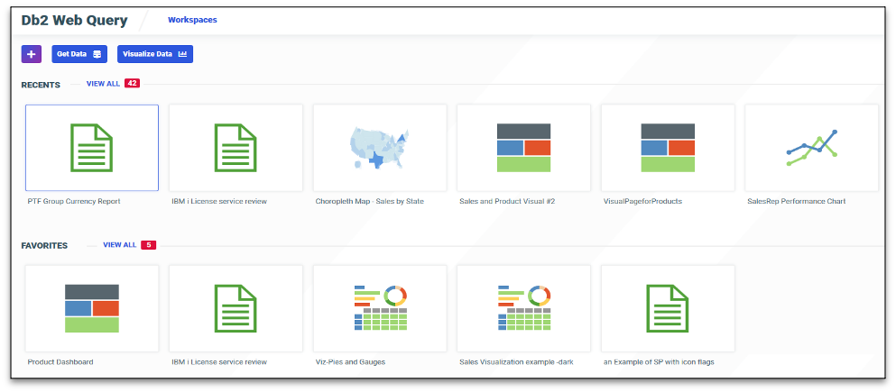
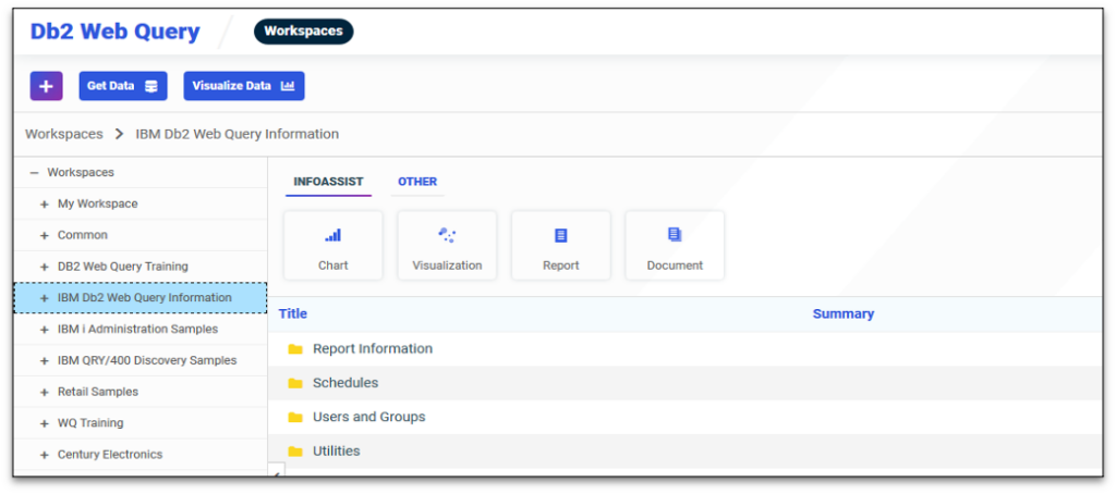
By Clicking Workspaces at the top of the panel, you will change the new interface to a layout similar to the older interface, where folders are shown, can be expanded or collapsed to show report names and where new report objects can be created. Figures 2 and 3 depict the new WQ interface where report development or execution is done.

IBM has provided a “Legacy Home Page” link in the new interface (under your user-id) to enable you to revert to the older interface if you choose.  You can actually use both in separate tabs of your browser if needed.

Creating Metadata From the SQL Procedure

Log into WQ with your user and password, bringing you to the Home page.

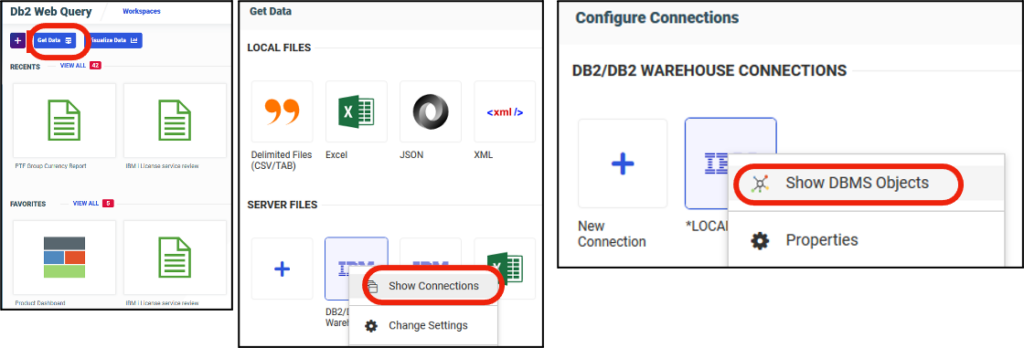
Click the Get Data icon to open the Metadata selection window.

On the Get Data panel, Right-Click Db2/Db2 Warehouse cli, then Click the Show Connections (see Figure 4).

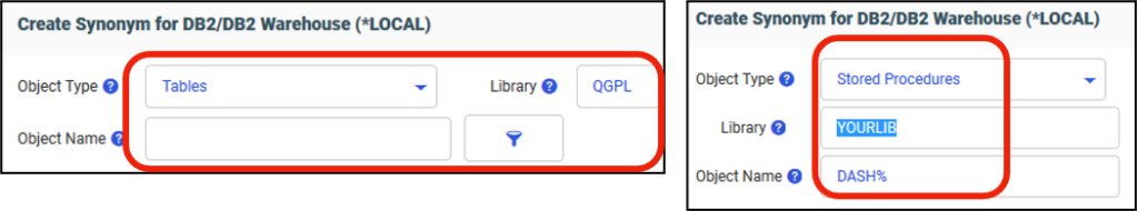
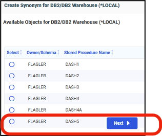
When the Create Synonym page opens, it defaults to TABLES, not SPs (see Figure 5). You’ll need to change the Object Type field from Tables to SPs, to locate available procedures.  Specify your library if your SP isn’t in QGPL. Enter a whole or partial Object name. I used DASH%, meaning, get a generic list of things like DASH. Note that if you enter DASH*, like a typical IBM i generic name, you’ll get no results. The % replaces * in this case. Press Next at the lower right of the window to have WQ look for matches. The result is a listing of objects matching what you entered. Select an item and press Next.

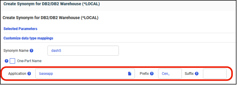
The second to last Create Synonym panel shows the synonym you’ll be creating and offers you a choice of where, in which WQ Application folder, to save the synonym (see Figure 6). You can optionally add a Prefix or Suffix  to the name. I added Cen_ as a prefix because the data is from the IBM sample Century Electronics data set.  When you press Next on this panel, the process to create a synonym takes place (see Figure 7).

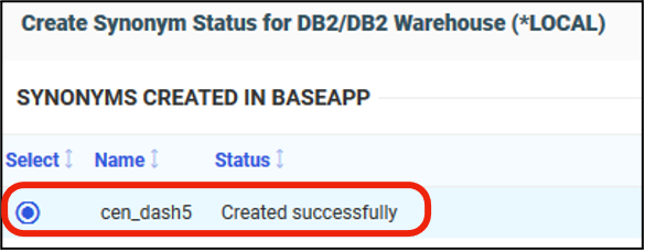
And, you should see a success panel (see Figure 8)

Using the Synonym in a Report

By creating the synonym, you’re ready to create a Web Query report using it. The name of your newly created synonym should appear (in our case cen_dash5) when you begin the process to author a new chart, report or visualization.

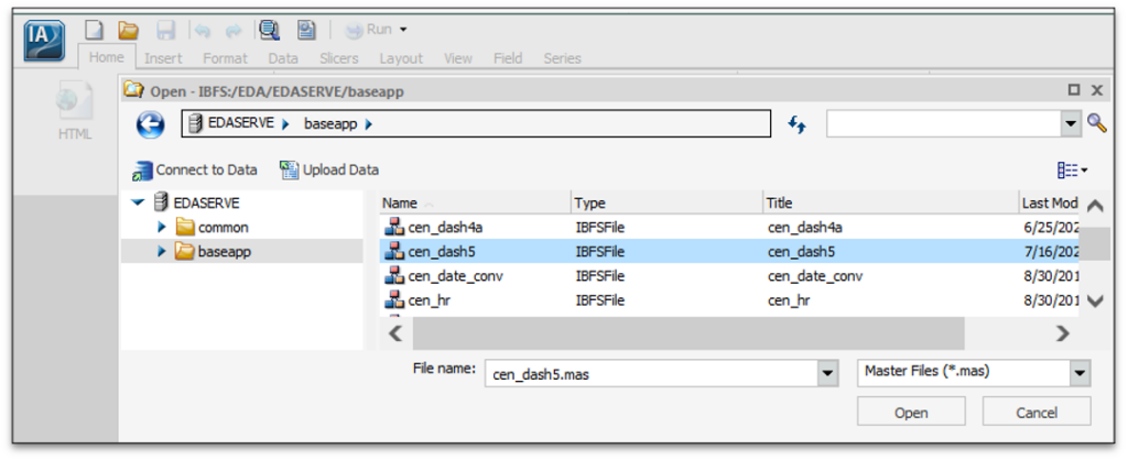
Launching the report designer (InfoAssist), you’d be prompted to select a data source and you’d see cen_dash5 in the list of available files (see Figure 9).

However, we want to enhance the metadata that was automatically created, to allow automatic drill down. We therefore must edit the file first, to make some minor changes.

Editing the Metadata

Return to the WQ Home page.

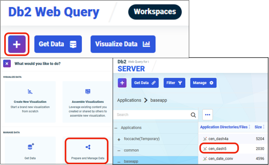
When you press the + icon to the Left of Get Data, you’ll be asked, “What would you like to do?” To edit an existing synonym, you click Prepare and Manage Data (see Figure 10). This will bring up a list of available synonym directories and files. On this list, locate the desired file (cen_dash5), right-click it, and specify Open.

The cen_dash5  file opens in the Metadata editor. Remember back to the SQL procedure? It had TWO result sets? In the metadata panel, you see ANSWERSET1 and ANSWERSET2 which represents those results (i.e.  records) to be returned by this synonym.

Figure 11: You can expand each ANSWERSET by clicking the + sign in front of the name, yielding a revised display with field details (see Figure 11).

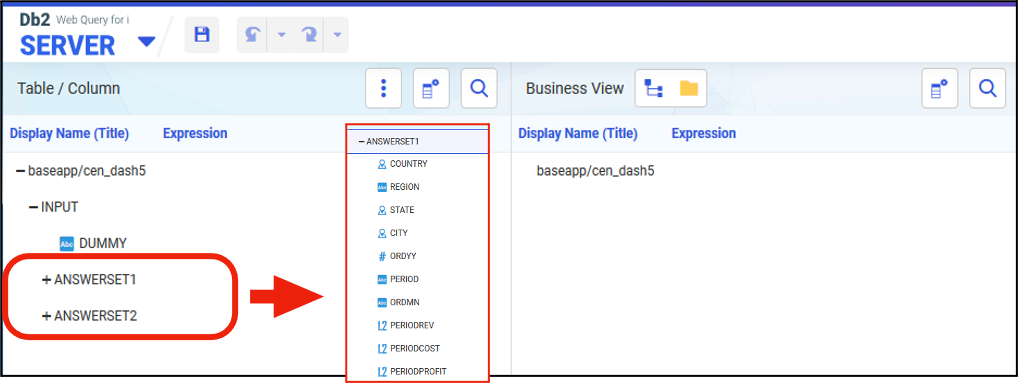
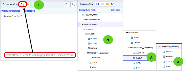
The SP’s C1 result, with grouping of fields as part of ANSWERSET1 are: country, region, state, city—four related geographic data fields. Assuming our report users want to drill down through the geography levels, all we need to do is modify the metadata to contain those fields under a geography hierarchy. In the center of the metadata editor, you’ll see text saying Click Create Default to populate the business view. 

Pressing that CREATE DEFAULT icon (1) updates the panel, showing that the metadata editor has done some work for you (see Figure 12). The Editor placed fields in the view and it identified some geographic fields as a hierarchy (2). However, because Region is not a “standard” geographic element as are country and state, it didn’t move the field and we have to do it manual by dragging region to a position between COUNTRY and STATE (3). Finally, by right-clicking and renaming the hierarchy, users might more easily understand this (4), so we change ANSWERSET1_Geography to Geographic_Hierarchy.

When the metadata changes have been made, click the save icon and exit the metadata editor. Your synonym will be ready to use.

Back at the Home page, we begin a new report by clicking Report, the InfoAssist designer opens, prompting you to select a data source and by choosing cen_dash5, we’ll see the available fields (see Figure 13).

We see the two answer sets, and note when Answerset1 is expanded, we see the Geographic_Hierarchy we created, containing the four fields. Note the small dots in their icons depicts the levels of the hierarchy.

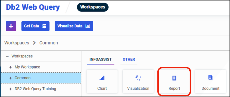
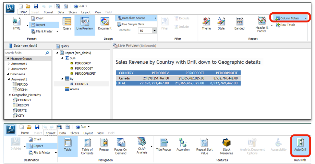
Figure 12: Dragging Country and the three numeric fields onto the canvas, we can very rapidly preview a new report for Sales Revenue. By clicking Column Totals, we add a grand total line. Clicking Format and Auto Drill will enable WQ to turn on drill down by country, to region, etc. By clicking Header & Footer, we can add a title (see Figure 14).

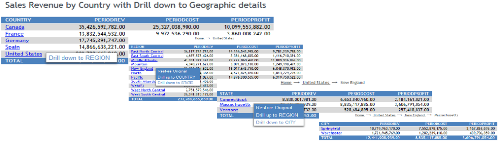
When run, the report depicts summary data for country and has a hyper-link on country, enabling us to drill to the region level, clicking region takes us to state, etc. (see Figure 15).

Visual Representations of Data

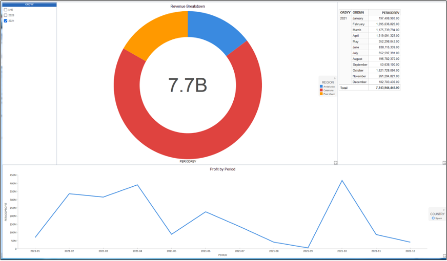
Similar techniques can be applied to charts in Web Query. Consider an InfoAssist Visualization utilizing the same data source (Figure 16). It contains three panes, each depicting data from the procedure, presented differently. The page will interactively recalibrate, based upon selections, filtering or drilldown in one of the areas.

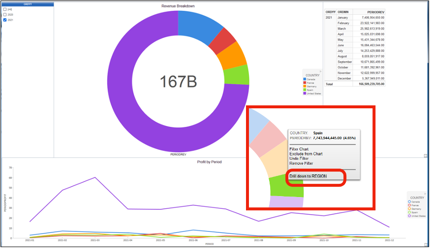
For example, by selecting the pie slice for Spain (Figure 17), drilling to region, we obtain a new view. Data analysts can work with data this way, to draw conclusions, plot strategies and discover facts that reports couldn’t show.

New Visual Data Pages

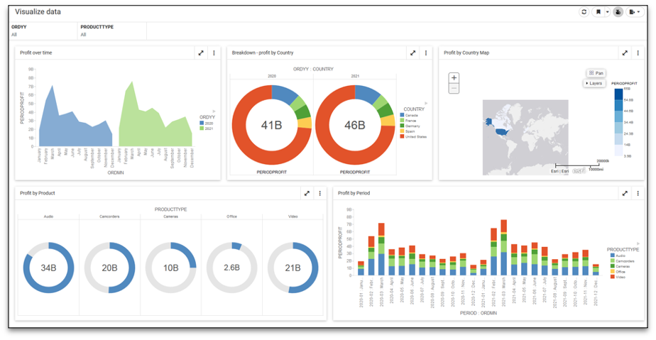
In Version 2.3, the visual capabilities were enhanced so it’s easier to create a page with multiple containers, (Figure 18). These visualizations are dynamic, again allowing for exploration of data. A picture can’t do it justice, but in this example, we see a multi-pane visualization with a selection for filtering by year and products. It depicts profit information in a variety of ways. As the user changes the year, the top three charts change. When product is changed, the bottom charts recalibrate.

As the user lassos a country pie slice to filter the chart in Figure 18, the charts and map change to reflect the lassoed data subset (Figure 19). Data can be included or excluded in this manner, making insights possible that textual reports cannot match.

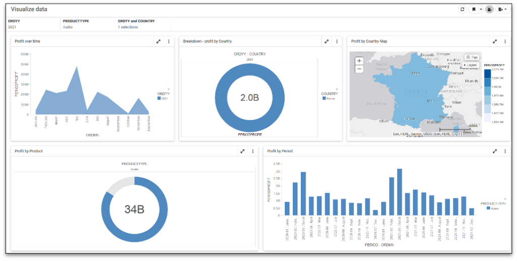
I’ll leave you to consider how these powerful tools can accelerate decision-making in your organization, but it sure beats reports we used to do with RPG programs or Query/400!

---